
- Published on
How to Read Logistic Regression Output
- Authors

- Name
- Isacar Racine
- @isacarracine
A model tells you an employee's chance of staying is 1.60.
That should stop you, because a chance cannot be bigger than 1. Nothing errored. The code ran, the number came out, and it went in the deck.
I have made that exact mistake. It is one of four things that go wrong when reading logistic regression output, and the reason they keep happening is that none of them break anything. The code runs fine. The number is just not the number you think it is.
Part 5 of a six-part series on regression. Previously: the R-squared trap.
Why you can't just use ordinary regression
Ordinary regression predicts a number that can be anything. Height, price, miles per gallon.
Now try predicting whether a customer churns. The answer is yes or no, which you write as 1 or 0, and you want the model to give you a chance somewhere between them.
Feed that to ordinary regression and three things break:
- It happily predicts −0.3 and 1.4. There is no such thing as a −30% chance.
- Its error bars are wrong everywhere, because a coin that lands heads 50% of the time is far more unpredictable than one that lands heads 99% of the time. Ordinary regression assumes they're equally unpredictable.
- Its residuals can't behave, because the actual answer is only ever 0 or 1.
Logistic regression fixes the first problem by squashing. It runs the same straight-line calculation you already know, then pushes the answer through a function shaped like a stretched S, which flattens out as it approaches 0 at one end and 1 at the other. No matter how extreme the inputs get, the answer stays a legal chance.
That squash is called the link function, which is a formal name for "the thing that converts the straight-line total into the answer you want." Swap the squash and you get a different model for a different kind of outcome:
| Your outcome | Example | The squash is called | The model is called |
|---|---|---|---|
| Any number | Price, mpg | nothing, it passes straight through | ordinary regression |
| Yes or no | Churned, approved | logit | logistic regression |
| A count | Support tickets, defects | log | Poisson regression |
Ordinary regression is the row where the squash does nothing. It is not a separate technique.
Trap 1: an odds ratio is not a probability
This is where the 1.60 came from.
A chance is the number you want: 62 out of 100, so 0.62.
Odds are the same fact written as a ratio: 62 stayers for every 38 leavers, so 62/38 = 1.63. Bookmakers talk this way. Odds run from 0 to infinity, so a value above 1 is perfectly normal.
Log-odds are odds run through a logarithm, which stretches them out to run from minus infinity to plus infinity. Ugly to read, but it is the scale on which the model's straight line is actually straight. This is what logistic regression works in.
Here's a real model, predicting whether employees stay from how many products they own:
(Intercept)         0.47134
Num.Of.Products2   -1.57329
Three correct ways to say what that −1.573 means:
- Owning two products lowers the log-odds of staying by 1.573. True, and useless to anyone.
- It multiplies the odds of staying by 0.207. Undo the logarithm and you get this. It's called the odds ratio.
- It moves the chance of staying from 61.6% to 24.9%.
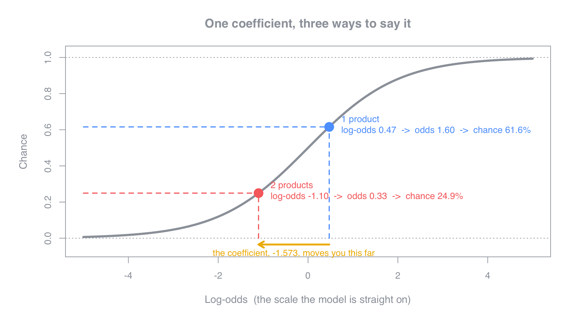
The curve is the squash. The coefficient moves you a fixed distance along the bottom axis, and the curve decides what that does to the chance. Near the middle a small shove moves the chance a lot. Out at the ends it barely moves it at all, which is exactly why one coefficient cannot correspond to one change in chance.
Trap 2: predict() returns log-odds unless you ask for type = "response"
Ask R for a prediction and it answers in log-odds, because that is the scale the model works in. It does not warn you.
predict(model1, newdata = e)                     # 0.4713  <- log-odds
exp(predict(model1, newdata = e))                # 1.6021  <- odds
predict(model1, newdata = e, type = "response")  # 0.6157  <- the chance
There's the 1.60. It's odds, and odds look enough like a chance to sail through review, right up until one comes out above 1.
Python has the same three scales and the opposite default, which is its own trap:
model1.predict(e, linear=True)   # 0.4713  <- log-odds
model1.predict(e)                # 0.6157  <- the chance (default)
Trap 3: the fit test runs backwards
Every p-value so far has meant the same thing: small is exciting. A small p-value says you found something.
Logistic regression comes with a goodness-of-fit test, and it is upside down.
The question it asks is "does this model fit the data?" and it assumes the answer is yes until proven otherwise. So a small p-value means your model does not fit. Here, you want a big one.
df <- nrow(rawdata) - length(coef(model1))
pearres <- residuals(model1, type = "pearson")
1 - pchisq(sum(pearres^2), df)
Two models on the same employee data:
| Fit test p-value | Verdict | |
|---|---|---|
| One predictor | ≈ 0 | does not fit |
| All predictors | 0.67 | fits |
Two more things about this test. First, the one-predictor model was significant overall and a bad fit at the same time. Those aren't contradictory. "At least one predictor carries signal" and "the model reproduces what actually happened" are different claims.
Second, and more important: this test needs repeats. It works by comparing what happened against what the model expected, within groups of rows that share identical predictor values. No repeated rows, no groups, no test.
How do you know it's broken? The two versions of the test disagree wildly. On a concrete-strength model I got this:
Deviance version: p = 1      (perfect fit)
Pearson version:  p = 0      (total failure)
Same model. When you see that, don't pick the answer you prefer. Neither is valid, and the diagnosis is not enough repeats.
Trap 4: overdispersion, and why dispersion should sit near 1
Ordinary regression estimates how noisy your data is. Logistic regression does not get to. Its maths forces the noise to a fixed level determined by the chances themselves.
Real data is often noisier than that, usually because rows cluster in ways you didn't model. Employees within the same manager. Customers within the same city.
The check is one number, called the dispersion:
model1$deviance / model1$df.residual
It should be about 1. That's what the model assumes. Bigger means your data is more scattered than the model believes, which is called overdispersion.
| Dispersion | What it means |
|---|---|
| ≈ 1 | as expected |
| 1.5 | already worth acting on |
| > 2 | clearly a problem |
The two employee models came in at 3.85 and 1.01. The first is badly overdispersed. The second is about as close to textbook as real data gets.
The fix is one word in your model: family = quasibinomial instead of binomial. That rescales the error bars and leaves the coefficients alone. For counts, quasipoisson does the same, and negative binomial regression is the sturdier option.
How to read logistic regression output in R
| What you see | What it means | What to do |
|---|---|---|
| Estimate | Change in log-odds | Exponentiate it for an odds ratio |
z value | Estimate over its error bar | Same idea as a t-value, different table |
Pr(> z ) | The p-value | Small means "probably real" |
| Null / Residual deviance | Badness before and after your predictors | A big drop means they're pulling weight |
| Fisher Scoring iterations | How many tries it took to fit | Above about 8, something is straining |
| Dispersion | Extra scatter | Should sit near 1 |
Seven things worth remembering
- Logistic regression is ordinary regression with a squash on the end. The adding-up part is identical.
- Chances, odds and log-odds are three different scales. Anything above 1 is not a chance.
- An odds ratio is not a chance ratio. Odds fell 79%, the chance fell 60%. Quote the one you mean.
predict()gives log-odds in R unless you ask fortype = "response". Python's default is the opposite.- The fit test wants a LARGE p-value, needs repeated rows, and is invalid if its two versions disagree.
- Check dispersion against 1, not 2. Overdispersion manufactures false positives.
- A coefficient can flip sign entirely when you add predictors. That one gets its own post.
For counts instead of yes/no, swap the logit squash for a log squash and everything above still applies, with overdispersion an even bigger worry.
Previous: the R-squared trap · Next: Variable selection, ridge, lasso, elastic net
See also: 15 ways to misread your own regression model.
Get the next one
Posts on data, analytics and the judgment calls that decide whether a model gets trusted.